


TAKEAWAYS
We accountants love templates because reusable templates save time. Train Excel right once, and it will repeat the task for you subsequently. One key aspect when creating templates is to consider scalability. A good template should adapt to varying amounts of data, minimising human intervention when scenarios change.
For the longest time, since I first used Excel, formulas only returned results in the very cell where you entered them; they didn’t automatically fill into other cells. This limitation meant that if you wanted to apply a formula to each line in a table, you had to manually copy it to every row. When new data was added, you had to update the formulas again, causing inefficiencies and increasing the chances of errors. Additionally, if your report table had a variable number of rows, you had to write formulas for the maximum number of lines you might need, which further limited scalability.
Excel introduced dynamic array formula functionality in Microsoft 365. Beyond addressing the inefficiencies mentioned above, let’s explore its benefits and how to apply it to accounting use cases.
Dynamic array formulas in Excel are a type of formula that can return multiple values simultaneously. Unlike traditional formulas that output a single value in one cell, dynamic array formulas can spill their results into multiple cells. This feature allows for more versatile and powerful data manipulation and computation – a must-know if you are building templates for scalability.
There are three key aspects of dynamic array formulas in Excel:
1. Newer dynamic array functions
Excel introduced several new functions designed to work with dynamic arrays. These include functions like FILTER, SORT, UNIQUE and SEQUENCE. These functions can generate arrays of values based on various criteria, and they automatically spill into the necessary range of cells.
2. Spill range operator (#):
Excel introduced the spill range operator (#) to work with dynamic arrays. This operator allows you to reference the entire spilled range of a dynamic array formula.
3. Range input:
Many Excel functions now allow you to select a range of cells as input rather than just a single cell. This capability enhances the flexibility and power of these functions. For example, you can now apply functions like VLOOKUP to entire ranges of lookup values in a single formula, making your calculations more efficient and less error-prone.
Let’s demonstrate this with a practical example: creating a lead schedule for audit working papers. Traditional Excel formulas would require you to copy a formula to each row of your schedule, and updating the data meant manually adjusting the formulas again. This process was time-consuming and prone to inconsistencies and errors.
Traditional method: Using VLOOKUP
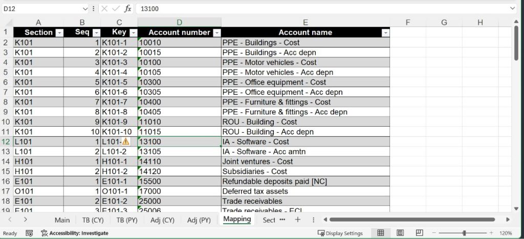
Consider a lead schedule for audit working papers where you need to get a list of account numbers mapped to a particular lead schedule (K101 for property, plant and equipment, for example), then look up the account numbers from the chart of accounts for their descriptions.
VLOOKUP only returns one result regardless of how many matches you have in the lookup table, and we usually have more than one account mapped to a single lead schedule. This makes it impossible for traditional lookup functions to return all relevant account numbers without complicated workarounds. So, the most practical and straightforward solution was to do an auto-filter in the lookup table, then copy and paste the relevant account numbers into the lead schedule template.
Then, you can use a VLOOKUP function to retrieve the account names from the chart of accounts. If you have more than 10 accounts (as in this example), make sure you copy the formula in cell C7 to all the rows.
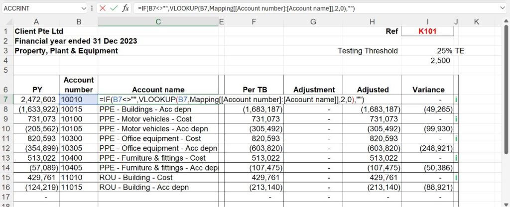
Note: If you are wondering how to make reference to data by calling the column header, you can find out more from Microsoft’s official documentation on structured referencing.
Modern method: Using FILTER
Now, let’s use the dynamic array function FILTER for the same task:
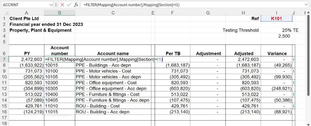
In cell B7, enter the filter function: =FILTER(Mapping[Account number],Mapping[Section]=I1).
When more than one result is found, this formula will spill the results into multiple cells, showing all account numbers associated with the section specified in cell I1 of the lead schedule.
To retrieve the account names in column C, you can use XLOOKUP (or VLOOKUP) in cell C7. To make XLOOKUP a dynamic array formula, instead of referring to our lookup value in cell B7, let’s add a # sign behind B7. This makes reference to the entire spill range starting from cell B7.
If you provide a range input to a function argument (for example, lookup_value of XLOOKUP) that originally only accepts a single cell reference, the formula will automatically spill. With this functionality, if the FILTER function in cell B7 returns more account numbers (or fewer), the XLOOKUP will adjust accordingly as well.
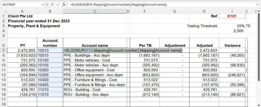
With this setup, the XLOOKUP function will dynamically adjust to the number of account numbers returned by the FILTER function in B7, ensuring that all relevant account names are retrieved and displayed in column C.
This is how you can do it for columns F, G and H:
Cell F7: =SUMIFS(TB_CY[Net],TB_CY[Account number],B7#)
Cell G7: =SUMIFS(Adj_CY[Net],Adj_CY[Account number],B7#)
Cell H7: =F7#+G7#
With this setup, you only need to copy this sheet and change I1 to another section to populate data for the next section. There are no complicated workarounds or manual filtering of relevant account numbers.
Here are a few other dynamic array formulas you might find useful. You can explore their functionality at your convenience:
UNIQUE: Returns a list of unique values from a range or array
SORT: Sorts the contents of a range or array
SEQUENCE: Generates a list of sequential numbers in an array

1. Function arguments accepting ranges:
This might not be intuitive. In column H, we would typically use =SUM(F7:G7). When adding a # operator after F7 and G7 (=SUM(F7#:G7#)), you might expect it to automatically spill through H16. However, it will not. Why?
The SUM function accepts ranges as its arguments. So, when you add # operators to the references, SUM will interpret it as if you want to sum the entire ranges where the spill range ends, making it equivalent to =SUM(F7:F16, G7:G16).
The formula will only auto-spill when the argument originally only accepts a single cell reference. That is why we use =F7#+G7# instead of SUM.
2. Dynamic array references:
You can’t use the spill range operator (#) to reference cells that are not part of a dynamic array result. Only dynamic array formulas produce spill ranges that can be referenced with the # operator.
3. Spill blocking:
If there’s existing data in cells where a dynamic array would normally spill, you’ll get a #SPILL! error. It’s important to ensure the spill range is clear to avoid this error.
4. Performance considerations:
Dynamic arrays are also more efficient for user time and maintenance, as they automatically adjust to changes in data size. Functions like UNIQUE, FILTER, and SEQUENCE can perform tasks more efficiently than traditional workarounds, making dynamic arrays a powerful tool for various scenarios.
However, for extremely large datasets or complex operations (for example, using FILTER or SORTBY on large tables), dynamic arrays might cause performance issues.
It has been a long wait for Excel fans, but dynamic array formulas are finally here, not only matching but in many ways exceeding similar features that have long existed in Google Sheets. These powerful tools allow accountants to handle data more efficiently and accurately, offering capabilities that go beyond what was previously possible in spreadsheet applications.
Dynamic arrays provide the ability to create scalable templates that adapt effortlessly to varying data sizes and complexities. While they are powerful, dynamic arrays require some learning and adjustment for users accustomed to traditional Excel formulas. However, the time invested in mastering these new functions will pay off through reduced manual updates, fewer errors, and more reliable financial reports.
Embrace dynamic arrays to streamline your accounting processes, to ensure your work remains efficient and future-proof.
Have you read the article “XLOOKUP Or VLOOKUP ”? It explores which lookup function works best for accountants, and why.
Ng Xian Hui, CA (Singapore), is Founder & Director of Backbone Pte Ltd.
